PROcess Safety TASK

Wellhead Injection Line Hazards

What is the Wellhead Injection Line?

A Wellhead Injection Line is also known as an injection flow line, is a pipeline used to transport fluid from surface facilities to an injection wellhead for various purpose, such as fluid disposal, enhanced oil recovery (EOR), or etc. Unlike production flow lines that transport fluids from WH to processing facilities.

Hence, the component of fluids from Wellhead Flowline and Wellhead Injection Line are difference. For example, the water injection may involve injecting produced water or treated seawater for reservoir pressure maintenance of EOR purpose. Gas injection may involve injecting natural gas or carbon dioxide for EOR or reservoir stimulation.

What are general hazards of Wellhead Injection Line?

Injection flow lines shall be designed to handle the injection rate and pressure required for the specific injection application. However, failure of some devices such as control valve, pressure regulator, and etc. can post of significant hazards.

Undesirable Event	Cause	Detectable Process Condition
Overpressure	Blocked or restricted outlet Hydrate plug Upstream control valve failure Plugged formation	High pressure
Leak	Deterioration Erosion Corrosion Impact damage Vibration	Low pressure

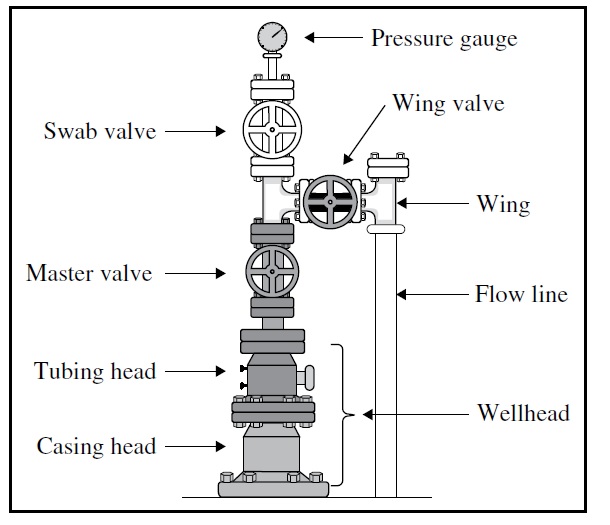
Safety Analysis Table (SAT) – Wellhead Injection Line

What are the Process Safety Device on Wellhead Injection Line?

Device	Location	Function
High Pressure Sensor (PSH) to shut off inflow	On the WH Injection source	– To alarm when abnormal pressure is found. – To prevent overpressure
Low Pressure Sensor (PSL) to shut off inflow	On the WH Injection source	– To prevent of leakage
Pressure Safety Valve (PSV)	On the WH Injection source (MAWP< shut off pressure from injection source)	– To prevent overpressure
Flow Safety Valve (FSV) or check valve	On the Injection line and near the WH	– To prevent the backflow from WH
Additional Shutdown Valve (SDV) and independent pressure sensor (*)	On the Injection line and near the WH	– To prevent backflow from WH

(*) Additional Shutdown Valve and independent pressure sensor is not required on the gas lift line if the system is protected at an upstream component and if they are not subject to backflow from producing formation.
(*) Additional Shutdown Valve and independent pressure sensor is not required if the injection line is for the purpose of injecting water and the subsurface formation is incapable of backflow hydrocarbon.
(*) If closing of SDV can cause of rapid pressure buildup to injection line, considering the shutdown of the injection source and using double FSV in lieu of an SDV.

Wellhead Flow Lines Hazards

What are the Wellhead Flow Lines (FL)?

Wellhead Flow Line (FL) หรือเรียกอีกอย่างว่า Production Flow Line (FL) คือระบบท่อที่นำส่งของเหลวที่ออกมาจากหัวเจาะ ไม่ว่าจะเป็นน้ำมัน ก๊าซ น้ำ หรือของเหลว Multiphase เข้าไปในส่วนการผลิตบนส่วน Topside

จากรูปข้างล่างระบบท่อ Flow Line (FL) จะต่อมาจาก Choked Valve กับ Wing Valve ที่ต่อมาจากด้านบนของตัว X-Mass Tree โดยจะใช้ Choked Valve ในการปรับอัตราการไหลและความดันเข้าสู่ Production Flow Line (FL)

และจากรูปก็จะมีในส่วน X-mass Tree หรือ Christmas Tee ซึ่งจะติดตั้งอยู่ด้านบนของ Wellhead หรือ หัวหลุมเจาะ โดยจะทำหน้าที่เป็นฐานในการติดตั้งวาล์วต่างๆที่กล่าวไว้แล้วข้างต้น ยังทำหน้าที่สำคัญเป็นตัวยึดแขวนระบบ Tubing ที่ถูกส่งลงไปในหลุมเจาะ Well

What are the general hazards of Flow Lines?

ในการวิเคราะห์ Flowline (FL) เราสามารถวิเคราะห์แยกออกเป็นส่วนย่อยๆ Segment ได้ โดยอาจจะแยกเป็นระดับความดันต่างๆ

ดังนั้นจะเห็นได้ว่า Process parameter ที่มีความสำคัญต่อระบบ Flowline (FL) คือความดัน โดยตารางข้างล่างได้สรุป สาเหตุของปัญหาที่เป็นไปได้ที่จะก่อนให้เกิดปัญหาทางด้านความดัน ทั้งก่อให้เกิดความดันสูง และความดันต่ำลง

Undesirable Event	Cause	Detectable process parameter
Overpressure	Blocked or restricted line Downstream choke plugged Hydrate plug Upstream flow control failure Changing well conditions Closed outlet valve	High pressure
Leak	Deterioration Erosion Corrosion Impact damage Vibration	Low pressure

Safety Analysis Table (SAT) of Flow Line Segment

Process Safety Devices

ในแง่ของการรักษาความปลอดภัยของระบบท่อ Production Flow Line (FL) โดยพื้นฐานที่สุด คือ ค่าการออกแบบความดัน หรือ Design Pressure ควรจะต้องออกแบบให้สามารถทนต่อความดันและอุณหภูมิสูงสุดที่มีโอกาสเกิดขึ้นได้จากหลุมเจาะ

รวมถึงเครื่องมือรักษาความปลอดภัยอื่นๆ เพื่อช่วยสนับสนุนการทำงานและเป็นระบบสำรองเพื่อควบคุมความดันให้อยู่ในเกณฑ์ที่ยอมรับได้ ก็มีอยู่ด้วยกันหลายชนิด เช่น ระบบป้องกันความดันสูง ระบบป้องกันความดันต่ำจากการรั่วไหล วาล์วระบายความดัน วาล์วความคุมอัตราการไหล เป็นต้น

Device	Location	Function
High Pressure Switch (PSH) to shut in the well.	Downstream WH, on each FL (MAWP>SITP)	– To detect abnormal high pressure i.e. malfunction of choke valve. – To prevent overpressure situation
Low Pressure Switch (PSL)	Downstream WH, on each FL (Length >3meter)	– To detect leakage in any FL.
Pressure Safety Valve (PSV)	Downstream WH, on each FL (MAWP<SITP)	– To prevent overpressure situation
Flow Safety Device (FSV) or check valve	Final FL segment	– To prevent the backflow
Additional independent Shutdown Valve (SDV) with PSH sensor*	Downstream WH, on each FL (MAWP<SITP)	– To prevent overpressure situation (Alternative PSV)

MAWP is Maximum Allowable Working Pressure
SITP is Shut-In Tubing Pressure which is the pressure of the fluid in the tubing after the well has been shut in for a period of time.
(*) Additional independent shutdown valve can be considered when it is adequate to allow sufficient time for closing SDV before exceeding the MAWP.

Climate Change

Climate change refers to long term changes in temperature, precipitation, wind patterns, and other atmospheric conditions on the Earth. It is primarily driven by human activities, such as the burning of fossil fuels (coal, oil, and natural gas), deforestation, and industrial processes, which release greenhouse gases (GHGs) into the atmosphere.

The most significant greenhouse gas is carbon dioxide (CO2), but others include methane (CH4), nitrous oxide (N2O), and fluorinated gases.

What is the Decarbonization?

Decarbonization refers to the process of reducing or eliminating carbon dioxide (CO2) emissions, particularly those generated by human activities. The goal of decarbonization is to mitigate the impact of climate change by decreasing the concentration of greenhouse gases, such as CO2, in the Earth’s atmosphere. The main focus of decarbonization efforts is often on sectors that are significant contributors to carbon emissions, such as energy, transportation, industry, and agriculture.

Key strategies for decarbonization include.

Transition to Renewable Energy: Shifting from fossil fuel (coal, oil, and natural gas) to renewable energy sources (solar, wind, hydro, geothermal) is a crucial step in reducing carbon emissions from the energy sector.
Energy Efficiency: Improving energy efficiency in buildings, transportation, and industrial processes can significantly reduce overall energy consumption and consequently, emissions.
Carbon Capture and Storage (CCS): Technologies that capture CO2 emission from industrial processes or power plants before they are released into the atmosphere can help prevent the greenhouse gas from contributing to global warming.
Electrification: Transitioning from fossil fuel-powered vehicles to electric vehicles and using electricity instead of fossil fuels for heating and industrial processes can contribute to decarbonization.
Reforestation and Conservation: Forests act as carbon sinks, absorbing and storing carbon dioxide. Protecting existing forests, reforesting areas, and promoting sustainable land use practices can enhance carbon sequestration.

Climate Risk Assessment

Climate Risk Assessment is a process that involves evaluating and understanding the potential risks and opportunities associated with climate change for businesses, organizations, communities, and other entities. This assessment aims to identify how climate-related factors, such as extreme weather events, regulatory changes, and shift in market dynamics, could impact various aspects of an entity’s operations, finances, and overall resilience. Key components of a climate risk assessment typical includes.

Physical Risk: Assessing the direct impacts of climate change on assets, infrastructure, and operations. This may include the risk of extreme weather events (e.g. hurricanes, flood, droughts), sea-level rise, and changes in temperature pattern.
Transition Risk: Evaluating the risks associated with the transition to a low-carbon economy. This involves considering regulatory changes, technological advancements, market shifts, and other factors that may affect the value of assets or the cost of doing business.
Regulatory Risks: Examining the potential impacts of new or evolving regulations related to climate change, emissions, and environment sustainability. Changes in environmental policies can have significant implications for certain industries.

Guideline to minimize failure of field devices – SIL Verification Study

Appendix B.10, Field devices of ISA-S84.01, Application of Safety Instrumented Systems for the Process Industries has presented the list of potential failures in the sensors system for reference such as;

Primary sensing elements are prone to failure due to the extreme process conditions;
Process connection faults;
Accidentally isolation of the process connection;
Fluid properties go worst such as Fouling, Corrosion, High viscosity, Clogging, and Pulsation;
Wiring errors;
Environmental-mechanic issues such as overheating, freezing, and high vibration.
Environmental-electric issues such as earthing and bonding damages.
Adverse weather conditions such as lightning, and flooding.
Environmental-radiated rays such as RFI/EMI, and X-ray.

The typical failure causes the deficient functionality of the components of the final element (valve) as follows.

Damages output switch from the logic solver;
Damages the solenoid valve used to feed and vent the power air or hydraulics;
Broken of the feed and vent tubing to the actuator
Malfunction of the actuator itself
The stuck position of valve steam and seat

Design for fail-safe operation

Fail-Safe Design: A fail-safe system is designed to revert to a predetermined safe state when a failure occurs. This means the designer should design sensors and final elements to result in fail-safe responses to their most likely failure modes.

However, the review of spurious trip rates to see whether they are acceptable shall be performed. A general practice of the fail-safe design of the field device is as follows.

Sensor contact shall be designed to close during normal operation and will open when fails.
Output contact shall be designed to close and to be energized for normal operation and de-energized-to-trip design. Actually, the standard allows to use of energized-to-trip design, but it is required to achieve a high safe fraction.
The system shall trip when the electrical wire is damaged.
The final valve shall move to the trip position (fail-safe) on the air failure.
If the SIS signal fails, it shall drive the final to the trip position.
Typically, a signal < 4 mA is used for tripping the final valve when the sensor is failed.

Separation of sensors from BPCS

Separation: The separation of BPCS (Basic Process Control System) and SIS (Safety Instrumented System) allows for more accurate execution of the situation and allocation of risk. The BPCS is designed to handle routine process control, while the SIS addresses specific safety-related risks. The reasons for not sharing the devices between BPCS and SIS are as follows.

The potential of common cause of failure
Loss of the opportunity to have multi number of layers of protection
Higher failure frequency
Risk to create confusion for normal routine maintenance and testing for maintaining the safety integrity.

The above illustrates the concept of sharing the level transmitter to control and prevent the gas blow-by due to loss of liquid level in the upstream pressure vessel.

Separated sensors for controlling and tripping

The above illustrates the concept of the separation of the level transmitter to control (LT1) and isolate the SDV valve (LT2) that can prevent the gas blow-by due to loss of liquid level in the upstream pressure vessel.

Diagnostics

Diagnostic functions refer to the capabilities of a system to monitor and assess its own health and performance. It can be considered a self-testing technique. Diagnostic features are designed to detect faults, failures, or deviations from expected behavior within the system. Hence, a high level of diagnostic coverage will convert many potentially dangerous failure conditions into a safe condition with an alarm or safe shutdown.

Proof testing cannot be claimed as a diagnostic due to the frequency of proof testing is very low compared to the potential demand.

Sensor diagnostics:

An example of sensor measurements such as pressure transmitters, level transmitters and etc. Here are some common diagnostic techniques for sensors.

Self-Test Capability: Modern sensors are equipped with built-in self-test capabilities.
Redundancy: Redundancy enables fault detection by comparing the outputs of multiple sensors. If one sensor provides a significantly different reading from the others, it will indicate a fault.
Signal Quality Monitoring: An example of some situations such as sudden spikes, noise, or erratic behavior in the signal will indicate sensor malfunction.
Comparative Monitoring: Deviation from the expected values can be indicative of sensor drift, degradation, or failure.

Final Element diagnostics:

An example of the final element is the shut-off valve which is required for online testing but it cannot be tested or closed during plant normal operation. Diagnostics provide a prove that the valve is still working properly. Below are the diagnostic test methods for the final element.

On-line trip testing: Actually, this method is a proof test, not a diagnostic test but to perform this technique, the valve must be equipped with the provision of bypasses.
Position Feedback Monitoring: The logic solver generates an alarm if the valve position does not match the command.
Stroke Time Monitoring: Deviation in stork time can indicate issues such as sticking or binding in the final element.
Partial Stork Testing (PST): PST intentionally tests a portion of the stroke of the final element without putting the entire system at risk.
Leakage Detection: This technique requires to use of additional measurement for monitoring for any leakage past the final element.

Redundancy in sensors and final elements

Redundancy helps in mitigating the impact of component failures. If service one component fails, the redundant component(s) can take over, maintaining the functionality of the system. The system can continue to operate even in the presence of failures.

IEC 61508 part 2 places an upper limit of the SIL that can be claimed which depends on the following factors.

Hardware Fault Tolerance (HFT);
Safe Failure Fraction (SFF)

Diversity

Diversity means using different types of sensor measurements or different final elements to achieve the same result. The objective is to minimize the possibilities of common cause failure or systematic errors.

Type of Fire – QRA

การศึกษาประเภทของไฟในกระบวนการประเมินความเสี่ยงเชิงปริมาณ Quantitative Risk Assessment (QRA) เป็นสิ่งสำคัญมาก เพราะนำไปสู่การวิเคราะห์ผลกระทบ Consequence Analysis (CA) ประเภทต่างๆของไฟ ด้วยเนื่องเพราะปัจจัยในการเกิดไฟประเภทต่างๆ มีทั้งที่เป็นปัจจัยภายในและปัจจัยภายนอก

โดยปัจจัยภายในจะขึ้นกับชนิดของสารซึ่งผู้ออกแบบสามารถที่จะพึงประเมินได้เองตั้งแต่เริ่มต้นขบวนการ แต่ปัจจัยภายนอกที่จะขึ้นกับสภาพแวดล้อมภายนอกนั้น จะคาดการณ์ผลลัพท์ที่สมบูรณ์นั้นค่อนข้างยาก ทั้งนี้เราสามารถลดความผิดพลาดที่อาจจะขึ้นโดยข้อมูลอ้างอิงจากภายนอก

ที่กล่าวข้างต้นเพื่อชี้ให้เห็นจุดที่ยังไม่สมบูรณ์ หรือจุดที่ยังพัฒนาต่อไปได้อีก ของระบบการเลือกประเภทของไฟที่อาจจะเกิดกับสารประเภทต่างๆนั้นยังไม่ได้มีในโปรแกรมคำนวณในปัจจุบันเท่าที่ผู้เขียนทราบ

ทั้งนี้การเลือกประเภทการวิเคราะห์ผลกระทบ Consequence Analysis (CA) ผิด จะส่งผลต่อผลคำนวนผึงได้เรื่องความรุนแรง เช่น การแผ่รังสีความร้อน ความเป็นไปได้ของการเสียชีวิต หรือความเสียหายต่อโครงสร้างจากการสัมผัสกับไฟ เป็นอย่างมาก

แผนภาพข้างล่างเป็นตัวอย่างการเกิดไฟประเภทต่างๆ เช่น Jet Fire (JF), Flash Fire (FF), Fire Ball (FB), และ Pool Fire (PF) โดยมองจากลักษณะการรั่วไหลของสาร เป็นตัวแปรตั้งต้น เช่น รั่วไหลจากถังความดัน leakage รั่วออกมาจากถังแตก และถังระเบิดเป็นต้น

จะสังเกตุได้ว่าค่าความดันไอของสาร หรือ Vapor Pressure ไม่ได้ถูกนำมาพิจารณา ซึ่งโดยปกติค่าความดันไอของสารยิ่งมีค่ามากก็ยิ่งกลายเป็นไอได้ง่ายในบรรยากาศ แต่ในขณะที่รั่วออกมาสู่ภายนอกเป็นจำนวนมากนั้นก็ยังมีสารบางส่วนที่ยังอยู่ในสภาวะของเหลวได้

ในแง่การคำนวณความถี่ในการเกิดไฟประเภทต่างๆ ในการการศึกษา Quantitative Risk Assessment เราใช้วิธีแผนภาพต้นไม้ หรือ Event Tree Analysis (ETA) แผนภาพข้างล่างเป็นแผนภาพโดยสรุป โดยมีการรวมปัจจัยภายนอก เช่น ความเป็นไปได้ในการติดไฟเข้าไปด้วย

Pool Fire (PF)

Pool Fire หรือ บ่อไฟ หมายถึงไฟที่เกิดจากการจุดติดของสารที่ติดไฟได้ในรูปของเหลว (liquid flammable substance) มักจะเกิดในพื้นที่เปิดโล่ง ทำให้เกิดบ่อของเหลวที่กำลังเผาไหม้ ไฟประเภทนี้สามารถเกิดขึ้นในพื้นที่เฉพาะเจาะจงและพบได้บ่อยในโรงงานที่มีการจัดการกับของเหลวไวไฟ (flammable liquid) ดังนั้น ผลกระทบจากไฟในบ่อจึงมักใช้เพื่อกำหนดเขตปลอดภัยในสถานที่ on-site safety zone แทนที่จะใช้สำหรับความเสี่ยงในชุมชน

โดยผลกระทบหลักของ Pool Fire คือเรื่องการแผ่รังสีความร้อนสู่ตัวผู้ปฏิบัติงาน เครื่องจักร ฐานรากที่สำคัญ อาคารที่ทำงาน เป็นต้น

Flash Fire (FF)

Flash Fire (FF) หรือไฟไหม้แบบแฟลช คือไฟที่เกิดขึ้นอย่างกะทันหันและรุนแรงซึ่งเกิดขึ้นในระยะเวลาสั้น ๆ และแพร่กระจายอย่างรวดเร็วผ่านเชื้อเพลิงที่กระจาย เช่น ไฟวิ่งผ่านกลุ่มละอองของไอระเหยที่ติดไฟได้ Flammable vapor ดังนั้น เราสามารถพิจารณาไฟลุกไหม้แบบแฟลชว่าเป็นการเผาไหม้ของกลุ่มไอระเหยที่ไม่เกิดการระเบิด (Nonexplosive combustion of vapor cloud)

อันตรายหลักจาก Flash Fire คือการแผ่รังสีความร้อนและการสัมผัสกับเปลวไฟโดยตรง อย่างไรก็ตาม จากเอกสารที่มีอยู่ ผลกระทบจากการแผ่รังสีความร้อนมีความสำคัญน้อยกว่าผลกระทบจากการระเบิด เนื่องจากระยะเวลาของผลกระทบน้อยมาก ไม่กี่ส่วนของวินาที

แบบจำลองไฟไหม้แบบ Flash Fire ไม่ควรดำเนินการตามการแผ่รังสีความร้อนทั่งไปของ Stefan-Boltzmann Law เนื่องจากอาจมีข้อผิดพลาดมากเนื่องจากอุณหภูมิยกกำลังสี่ Q = σ * ε * A * T⁴ โดยทั่วไปแล้ว พื้นที่เกิดการเผาไหม้ของ Flash Fire จะถูกประมาณโดยการจำลองการกระจายของก๊าซที่ติดไฟได้ Flammable Gas Dispersion Modeling.

Jet Fire (JF)

Jet Fire (JF) เกิดขึ้นเมื่อก๊าซหรือของเหลวที่ติดไฟได้ถูกปล่อยออกมาผ่านช่องเปิดขนาดเล็กหรือการแตกหักในท่อส่ง ทำให้เกิดเปลวไฟที่มีความเร็วสูง Jet Fire จัดว่าเป็นมีความอันตรายเป็นพิเศษเนื่องจากความรุนแรงและศักยภาพในการแพร่กระจายอย่างรวดเร็ว

อย่างไรก็ตาม ผลกระทบของ Jet Fire คล้ายกับ Pool Fire คือผลกระทบจากการแผ่รังสีความร้อนในพื้นที่ใกล้เคียง เครื่องจักร ฐานรากที่สำคัญ อาคารที่ทำงาน เป็นต้น

Fireball (FB)

Fire Ball (FB) คือมวลทรงกลมของเปลวไฟที่เกิดจากการจุดติดไฟของวัสดุที่ติดไฟได้จำนวนมากพร้อมๆกัน โดย Fire Ball มักเกี่ยวข้องกับเหตุการณ์ระเบิดและสามารถก่อให้เกิดความเสียหายอย่างมาก

ตัวอย่างของสถานการณ์ Fire Ball คือไฟไหม้บนถัง LPG สถานการณ์นี้จะสร้างการเปลี่ยนสถานะอย่างรวดเร็วของ LPG จากของเหลวกลายเป็นไป เรียกว่าเกิด Rapid Phase Transition (RPT) ซึ่งของเหลวที่ถูกเก็บไว้เหนือจุดเดือดตามบรรยากาศจะเปลี่ยนเฟสเป็นไออย่างรวดเร็ว ทำให้เกิดการปล่อยพลังงานทันที หากความดันของมันเกินความดันที่ออกแบบไว้ มันจะรั่วไหลและเกิดไฟลุกไหม้ สิ่งนี้มักจะมาพร้อมกับลูกไฟขนาดใหญ่ที่เกิดจากการระเบิดของละอองฝอยของสาร

Characteristic of Ignition

จากรูปข้างบน จะสังเกตุพบว่าลักษณะของการติดไฟจะแบ่งออกเป็น ติดทันทีทันได Immediate ignition ติดหลังจากนั้น delayed ignition หรือไม่ติดไฟ โดยการติดไฟทันทีทันไดจะเกิดจากความร้อนที่เกิดขึ้นจากการเสียดทานในระหว่างการรั่วไหล โดยมากจะเกิดและเป็นสาเหตุให้เกิดไฟไหม้แบบ Jet Fire

แต่ถ้าเป็นการติดไฟภายหลังหรือ delayed ignition หมายถึง การรั่วไหลของสารไวไฟ ได้ไปสัมผัสกับความร้อนหรือประกายไฟภายนอก ซึ่งอาจจะมาจากอุณหภูมิพื้นผิวของอุปกรณ์ การเสียดสีของวัสดุ เป็นต้น ทำให้เกิดไฟย้อนกลับมาหาจุดที่รั่วอยู่ได้ โดยถ้าเกิดเร็วมากๆ ก็จะเกิด Flash Fire เป็นต้น

Mean Time To Failure (MTTF)

MTTF or Mean Time To Failure is a reliability metric used to estimate the average time that a system, component, or device is expected to operate before experiencing a failure. MTTF is often expressed in terms of hours.

The benefits of studying MTTF in the field of reliability engineering are the following;

Reliability Assessment: MTTF can present how well a system or component performs over time before experiencing failure;
Maintenance Planning: MTTF helps in planning maintenance activities. It allows maintenance teams to schedule preventive maintenance and the inspection period.
System Design and Improvement: MTTF data is necessary data for analyzing the contribution factor to system failure. Understanding the MTTF can enhance the overall reliability of a system.

It’s important to note that MTTF applies to repairable systems, meaning they can be restored to operation after a failure.

There are other metrics of reliability engineering such as Mean Time To Restore (MTTR), and Mean Time Between Failure (MTBF).

MTTF focuses on the average time a system operates before failure in repairable systems, meaning they can be restored to operation after a failure.
MTTR measures the average time it takes to repair a system and bring it back into operation.
MTBF represents the average time between consecutive failures in non-repairable systems. MTBF is commonly used for non-repairable systems where failures result in permanent damage.

Calculation formula

Basic calculations of the MTTF and MTBF are similar. They are calculated as the total operating time divided by the number of failures.

Example-1

DCS system failure time as the following table.

	Time to Fail (hours)	Mode
Failure 1	2425	Dangerous
Failure 2	3350	Safe
Failure 3	4520	Dangerous
Failure 4	1525	Safe
Failure 5	3200	Safe
Failure 6	4115	Dangerous

A DCS system has measured dangerous failure data from the above table.

First dangerous failure = 2425 hours;

Second dangerous failure = 7870 hours (3350 + 4520);

Third dangerous failure = 8840 hours (1525 + 3200 + 4115)

The average of these three dangerous failure is (2425 + 7870 + 8840)/3 = 6,378 hours or it can be calculated by (2425 + 3350 + 4520 + 4525 + 1525 + 3200 + 4115)/3 = 6,378 hours.

MTTF of a system

Toxic Gas Effects – QRA

Toxic Gas Effects analysis involves the study and assessment of the adverse effects of toxic substances on living organisms, ecosystems, or the environment.

There are several benefits to the assessment of toxic gas effects such as;

Occupational Health and Safety: This is to ensure the safety of workers. Especially, where employees may be exposed to hazardous gases.
Emergency Response: Quantifying toxic gases during emergency situations, such as chemical spills, or accidental leaks will help emergency responders take appropriate measures to protect on-site personnel and facilities.
Health Risk Assessment (HRA): Evaluate the potential health risks associated with exposure to specific toxic gases. This includes assessing the cumulative impact of multiple gases and determining the level of risk for individuals and populations.

Safety Consideration

Many useful measures are available to use as benchmarks for predicting the consequence of whether that exposure will result in injury or death.

Emergency Response Planning Guideline for Air Contaminants (ERPGs) issued by the American Industrial Hygiene Association (AIHA);
Immediately Dangerous to Life or Health (IDLH) level established by the National Institute for Occupational Safety and Health (NIOSH);
Threshold Limit Values (TLVs) established by the American Conference of Governmental Industrial Hygienists (ACGIH) including Short-Term Exposure Limits (STELs), Time-Weight Average (TWA), and Celling (C)
Permissible Exposure Limits (PELs) issued by the Occupational Safety and Health Administration (OSHA).

Level	Short Definition
ERPG-1	Max Conc. for 1 hr that causes mild adverse health effects.
ERPG-2	Max Conc. for 1 hr that causes irreversible or serious health effects.
ERPG-3	Max Conc. for 1 hr that causes life-threatening.
IDLH	Concentration that causes death or permanent adverse health effects.
TLV-STEL	Max Conc. for 15 min exposure without suffering
TLV-TWA	Average Conc. for continued exposure (40 hr/wk) without suffering
TLV-C	Conc. that should not be exceeded at any time.

Permissible Exposure Limit (PEL) provides three (3) levels, similar idea with the Threshold Limit Value (TLV), both standards provide TWA, STEL, and Celling value where the PELs are developed by OSHA but the TLV is developed by ACGIH.

Lethal Concentration (LC)

Lethal Concentration (LC) refers to the concentration of a substance at which a specific effect. It is a term commonly used in toxicology to describe the concentration of a substance that is lethal to a given percentage of test organisms.

LC 1%	The level concentration at which 1% of test organisms die.
LC 50%	The level concentration at which 50% of test organisms die.
LC 90%	The level concentration at which 90% of test organisms die.
LC 99%	The level concentration at which 99% of test organisms die.

Application

Example design criteria for designing Restricted Area and Impacted Area.

Equipment	Scenario	Criteria
Flare	Un-ignited toxic gas release, cloud dispersion from gas/two-phase or liquid accidentally releases	LC 1%
Flare	Emergency operation (ignited)	TLV-TWA
Flare	Flame out	LC 1%
Cold vent	Emergency operation	TLV-STEL
Blow out	Un-ignited release	LC 1%

Design criteria of Restricted Area

Equipment	Scenario	Criteria
Flare	Un-ignited toxic gas release, cloud dispersion from gas/two-phase or liquid accidentally releases	IDLH
Flare	Flameout	IDLH
Cold Vent	Emergency operation	IDLH
Blow out	Un-ignited release	IDLH

Design criteria of Impacted Area

Probability of Fatalities

The most common method to calculate the probability of fatalities can be represented by the probit function since the probit function (logarithm of dose) provides a much straighter line that is close to the typical dose-response curve. Below is the basic equation of the probit function

And below is the conversion table from probit variable to probability or percentage.

The probit functions are available for a variety of exposures, including exposures to toxic materials, heat, pressure, sound, and etc. Below is the probit function to estimate fatalities level for lethal toxicity.

Substance	a	b	n
Ammonia	-35.9	1.85	2
Benzene	-109.78	5.3	2
Carbon Monoxide	-37.98	3.7	1
Chlorine	-8.29	0.92	2
Sulfur Dioxide	-15.67	2.10	1

Thermal Effects – QRA

การศึกษาผลลัพธ์ของผลกระทบจากความร้อนในระหว่างการศึกษาความเสี่ยงเชิงปริมาณ Quantitiative Risk Assessment (QRA) หรือ ในการออกแบบต่างๆ ก่อให้เกิดประโยชน์ต่างๆ เช่น การปรับแต่งการออกแบบ การพิจารณาด้านความปลอดภัยสำหรับผู้ปฏิบัติงาน การเลือกวัสดุทนไฟ หรือการประเมินผลกระทบต่อสิ่งแวดล้อม เป็นต้น

รวมถึงถ้าผู้ออกแบบเข้าใจผลกระทบจากความร้อน เช่นการเพิ่มขึ้นของความร้อนส่งผลอย่างไรต่อการทำงานของเครื่องจักร เช่น Fire Water Pump, Transmitter, หรืออื่นๆ ก็เป็นสิ่งสำคัญสำหรับการรับรองความปลอดภัยของระบบและอุปกรณ์ที่เชื่อมโยงกัน

ซึ่งในบทความนี้จะจำกัดอยู่ที่ฝั่งตัวรับ Receptor ที่ไม่ว่าจะเป็นตัวบุคคลหรืออุปกรณ์ต่างๆที่มีโอกาสได้รับผลกระทบจากความร้อน

Safety Considerations

ในแง่ผลกระทบความร้อนที่กระทำต่อผู้ปฏิบัติงานที่หน้างาน ทาง International Standard ได้ให้แนวทางการพิจารณาไว้ดังนี้

โดยทาง API 521: Pressure-relieving and Depressuring system ได้ให้แนวทางผลกระทบในแง่ความเข้มของความร้อนต่อระยะเวลาที่ก่อให้เกิดความเจ็บแสบของผู้ปฏิบัติงานที่หน้างานไว้ตามตารางข้างล่าง

Radiation intensity (Btu/hr/ft²)	Radiation intensity kW/m²	Time to pain threshold
500	1.74	60
740	2.33	40
920	2.90	30
1500	4.73	16
2200	6.94	9
3000	9.46	6
3700	11.67	4
6300	19.87	2

Permissible Design Level (k) kW/m² (Btu/h.ft²)	Conditions
9.46 (3,000)	Maximum radiant heat intensity at any location where urgent emergency action by personnel is required. When personnel enter or work in an area with the potential for radiant heat intensity greater than 6.31 kW/m2, radiation shield and/or special protection apparel should be considered.
6.31 (2,000)	Maximum radiant heat intensity in area where emergency actions lasting up to 30s can be required by personnel without shielding.
4.73 (1,500)	Maximum radiant heat intensity in area where emergency actions lasting up to 2 – 3 mins can be required by personnel without shielding.
1.58 (500)	Maximum radiant heat intensity at any location where personnel can be continuously exposed.

Recommended Design Thermal Radiation for Personnel

ข้อมูลทั้งหมดข้างต้นถือว่าพนักงานสวมใส่เสื้อผ้าที่เหมาะสม เช่น หมวก Safety เสื้อแขนยาวที่ติดกระดุมที่ข้อมือ ถุงมือทำงาน กางเกงขายาว และรองเท้าทำงาน

นอกจากนี้ ตารางข้างต้นแนะนำเกณฑ์ทางความร้อน โดยไม่รวมรังสีจากดวงอาทิตย์ เพื่อกำหนดเขตห้ามเข้า Restricted Area หรือกำหนดความสูงของปล่องความร้อน

และผลกระทบของรังสีความร้อนต่ออุปกรณ์ เครื่องจักร แสดงไว้ในตารางด้านล่าง

Radiation Intensity (kW/m2)	Observed Effect
37.5	Sufficient to cause damage to process equipment
25	Minimum energy required to ignited wood indefinitelu long exposure
12.5	Minimum energy required for pilot ignition of wood, meting of plastic tubing
9.5	Pain threshold reached after 8 sec, second degree burns after 20 sec.
4	Sufficient to cause pain to personnel if unable to reach cover within 20 sec, however blistering of the skin is likely.
1.6	Will cause no discomfort for long exposure

Probability of Fatalities

วิธีที่พบบ่อยที่สุดในการคำนวณความน่าจะเป็นของการเสียชีวิต Probability of Fatality สามารถแสดงโดยฟังก์ชัน probit เนื่องจากฟังก์ชัน probit ที่แสดงในรูป Logarithm นั้น ให้ผลลัพท์คล้ายพฤติกรรมความเป็นจริง ที่ว่า “ยิ่งได้รับมาก รับนาน โอกาสการเสียชีวิตก็มีโอกาสที่สูง”

ตารางข้างล่างคือ ตารางแปลงค่าคำนวณ Y ที่ได้ออกมาเป็น โอกาสการเสียชีวิต Probability of Fatalities

ฟังก์ชัน probit มีให้ใช้สำหรับการสัมผัสกับอันตรายหลายๆ ประเภท เช่น การสัมผัสกับสารพิษ ความร้อน ความดัน เสียง และอื่นๆ ด้านล่างนี้เป็นฟังก์ชัน probit เพื่อประเมินระดับการเสียชีวิตจากปริมาณความร้อนที่กำหนดจาก Pool Fire และไฟลุกไหม้ทันที, Mudan (1984).

Example

Determine the thermal flux necessary to cause 50% fatalities for 10 second for exposure.

For t = 10 sec, I = 60.5 kW

Thermal Radiation Analysis

การแผ่รังสีความร้อนจากเหตุการณ์ไฟไหม้และผลกระทบจากความร้อนนั้น ความร้อนส่วนใหญ่มาจากการแผ่รังสีความร้อนซึ่งสามารถคำนวณได้ตาม Stefan-Boltzmann equation

อย่างไรก็ตาม สมการนี้ไม่สามารถนำไปใช้ในสภาพจริงได้ เนื่องจากอุณหภูมิของเปลวไฟแตกต่างกันทั่วทั้งเปลวไฟ มันไม่ใช่ค่าคงที่ เนื่องจากมีปัจจัยอื่นๆที่ส่งผลต่อการแผ่รังสีความร้อน เช่น ความเป็นเขม่า

ดังนั้นในการหาการถ่ายเทความร้อนและผลกระทบของมัน มักจะใช้แบบจำลองอยู่ 2 แบบ

Point Source Model
Solid Flame Model

Point Source Model

โมเดล point source ไม่ได้พิจารณาถึงรูปร่างของเปลวไฟ แต่สมมติว่าความร้อนเกิดจากจุดกำเนิดในรูปทรงกลม โดยทั่วไปแล้วสมการนี้จะแสดงผลลัพธ์แบบ conservative

สมการโมเดล point sources ที่นิยมใช้คือ API Method, Brzustowski และ สมการ Sommer

Solid Flame Model

การออกแบบโมเดลเปลวไฟแบบของแข็ง ได้ตั้งสมมติว่าเปลวไฟมีรูปร่างเป็นของแข็งที่ปล่อยความร้อนออกมาเฉพาะจากพื้นผิวเท่านั้น รูปร่างของเปลวไฟจะถูกนำมาพิจารณา อัตราการถ่ายเทของความร้อนจะถูกคำนวณเป็นฟังก์ชันของ พลังงานการปล่อยจากพื้นผิว Surface Emitting Power (SEP), ปัจจัยรูปร่าง, และการส่งผ่านของบรรยากาศ Atmospheric Transmissivity

API Method

วิธีการ API อ้างอิงจากการถ่ายเทของความร้อนจากแหล่งความร้อนแบบ Point Source และการแผ่รังสีความร้อนที่อนุญาตที่จุดรับ Allowable heat radiation วิธีนี้พัฒนาโดยวิธีของ Hajek และ Ludwig เพื่อกำหนดการแผ่รังสีของเปลวไฟไปยังจุดที่สนใจ มันเป็นแบบจำลองแหล่งจุดที่ใช้ได้กับเปลวไฟแบบ Jet Fire ทั้งแบบ laminar flow และ turbulent flow

สมมติฐานหลักของวิธี API คือเปลวไฟจะถูกพิจารณาเป็นแหล่งจุดเดียวที่ตั้งอยู่ที่ศูนย์กลางของเปลวไฟซึ่งแผ่รังสีออกไปในทุกทิศทางจากศูนย์กลาง และอัตราส่วนของความเข้มของความร้อนที่ส่งผ่าน (Fraction of heat intensity transmitted) ถูกสมมติว่าเป็น 1.0

ตามที่อธิบายข้างต้น หนึ่งในปัจจัยที่มีผลต่อการถ่ายเทของความร้อนคือระยะทาง ที่หลายๆ โมเดลให้ความสำคัญ สำหรับโมเดล API ได้จัดเตรียมแผนภูมิอ้างอิงเพื่อกำหนดความสูงของเปลวไฟรวมถึงการยกตัวขึ้นดังนี้

ค่าแกน X จะได้จากการคำนวณความร้อนของสาร ลากขึ้นไปตัดเส้นตรงแล้วหักไปตัดแกน Y จะได้ค่าความสูงของเปลวไฟ ในหน่วย เมตร

และเมื่อพิจารณาผลกระทบของลมจากสิ่งแวดล้อมภายนอกต่อความเร็วของการไหลที่ออกจากรูหรือท่อ จะทำการเบี้ยวของเปลวไฟ กราฟต่อไปนี้จะถูกใช้

Example-1

Design the flare exclusion zone 6.3 kW/m² of the elevated flare stack height 33.3-meter, fraction of heat radiated 0.3, the maximum capacity at 34,056 m³/h and the heat radiation at flame is 6.3×10⁵ kW through the flare inside diameter 0.468 meter against the design wind velocity is 8.9 m/s. The material is hydrocarbon vapour, the average relative molecular mass of vapour is 46.1 and the flow temperature is 422 K.

Brzustowski and Sommer

The equation for the calculation of the heat flux at a given distance is the same as the API method above. Both methods are based on the single-point source. But Brzustowski and Sommer method is more preciously consider in the location of flame center shall upon the diffusion of a turbulent jet to the lean explosive concentration unit one.

The lower explosive limits of mixtures can be calculated using Le Chatelier’s rule as follows.

Then additional factors that need to be calculated for assessing the wind effects to flame geometry are the lower explosion limit concentration parameter and jet trust and wind trust parameter. Hence, the actual location of flame center can be determined via the below graph.

And lastly, Brzustowski and Sommer recommend the use of fraction of heat intensity transmitted (Tau) to correct the radiation impact. This is because of the environmental also can also absorb the heat about 10% to 20% over distance of 150 meter.

Fraction Heat Radiated (F) Factor

The F Factor or fraction of combustion heat radiated from a flame is the most important single parameter in the calculations of thermal radiation calculation.

Flare Design

ในการออกแบบปล่องเผาไหม้ หรือ Flare สามารถออกแบบได้ตาม International Standard ดังนี้

API STD 521, Pressure-relieving and Depressuring Systems ที่จะแสดงถึงวิธีการออกแบบความสูงที่ต้องการของหอเผาไหม Flare ด้วยสมการต่างๆที่กล่าวข้างบน
API STD 537, Flare Details for General Refinery and Petrochemical Services ที่จะอธิบายส่วนประกอบต่างๆของหอเผาไหม้ พร้อมทั้งระบบที่ควรจะมีเพื่อป้องกันอันตรายที่อาจจะเกิดขึ้น

Event Tree Analysis (ETA) – QRA

Event Tree Analysis (ETA) is a graphical tool used in Quantitative Risk Assessment (QRA) and decision analysis to evaluate the possible outcomes of a series of events. The overviews of how Event Tree Analysis (ETA) are as follows.

Identification of Initiating Event: The analysis starts with the identification of the initiating event (IE), which is the initial incident or condition that triggers the analysis such as LPG cylinder failure and LPG gas leakage.
Branching Events: From the initial event, the analyst develops a tree-like structure, with branches representing different possible outcomes or scenarios. Each branch represents a Possible Event (PE) or decision that may follow the initial event such as detected by the gas detector.
Probabilities: Along each branch, probabilities are assigned to different events or decisions
Endpoint: The analysis culminates in endpoints, which are the final outcomes or consequence outcomes of the event.

Example

A Diesel Oil (DO) tanker pumps excessive DO material to a storage tank than the available capacity due to the malfunction of level monitoring resulting in overfilling and releasing material to the working area via the venting system. This can lead to pool fire if ignited.

Based on the record, the frequency of refilling the DO is once per month, and due to the orientation training provided to the driver before performing the activities, the potential of human error to omit the liquid level during filling is 0.02. The potential that the driver will not detect a high-level alarm is 0.4. The potential of liquid pool fire is estimated at 0.01. The calculation of all the outcomes is as follows.

Compare between ETA and FTA

Event Tree Analysis (ETA) is often used in conjunction with Fault Tree Analysis (FTA), another technique in risk assessment. While FTA starts with an undesired event and traces back to its root causes, ETA starts with an initiating event and explores the possible outcomes and consequences.