Markov modeling is a mathematical modeling technique used to analyze and describe systems that undergo transitions between different states over time. Markov modeling is beneficial in reliability analysis for several reasons. It provides a systematic and mathematical approach to understanding the behavior of the system.
Benefit
State-Based Representative: Markov models allow the representation of a system’s reliability in terms of different states such as Operational State (Up), Failed State (Down), and Degraded State.
Dynamic Analysis: Markov models are particularly useful for systems with dynamic behavior, where transitions between states occur over time. This is valuable in analyzing complex systems where the reliability may change on the operational conditions, maintenance activities, or external factors.
Quantitative Analysis: The Markov models enable the quantitative assessment of the reliability of the system. It can be used to determine the steady-state availability, expected number of transitions, and mean time to failure.
Flexibility in Modeling: Markov models can be adapted to model various types of systems, including repairable and non-repairable systems.
Handling Complex System: Markov models are effective in handling complex systems with multiple components and failure modes. The model can be expanded to include various subsystems and interactions.
Sensitivity Analysis: Markov models allow for sensitivity analysis to identify critical components or states that significantly impact system reliability. This information is valuable for prioritizing resources.
Markov Modeling Steps
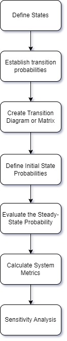
- Define States: Identify and define the different states of the system can be in such as operational, degraded, and failed.
- Establish Transition Probability: Determine the probabilities of transition from one stage to another. These transition probabilities are typically presented by a transition probability matrix (P), where Pij is the probability of transitioning from state i to stage j.
- Create a Transition Diagram or Matrix: Develop a visual representation of the Markov model using a state transition diagram or matrix.
- Define Initial State Probabilities: Specify the initial probability of the system being in each state at the start of the analysis. This information is represented by an initial state probabilities vector or transitioning vector.
- Evaluate Steady-State Probabilities: Determine the steady-state probabilities, which represent the long-term probabilities of the system being in each state.
- Calculate System Metrics: Once the steady-state probabilities are known, various system reliability metrics can be calculated such as mean time to failure (MTTF), and expected number of transitions between states.
- Sensitivity Analysis: Conduct sensitivity analysis to understand the impact of changes in transition probabilities on the overall system reliability. This will involve varying transition probabilities and observing their effects on the system metrics.
Markov Simple Transition Diagram
The simple of the Markov two-state transition and matrix are below. The states are “Operational (O)” and “Failed (F)”. The transition probability between these states is represented by a transition probability matrix (P).

- 1-POF is the probability of staying in the Operational State;
- POF is the probability of transitioning from Operational to Failed State;
- 1-PFO is the probability of staying in the Failed State;
- PFO is the probability of transitioning from a Failed State to the Operational; and

Example: Steady-State Availability
A repairable transmitter with one failure has a probability that the transmitter will fail 0.1 and once the failure is detected, the probability of the repair and recovery is 0.8. The Markov transition and matrix are the following. What is the Steady-State Probability? What is the Steady-State Availability?


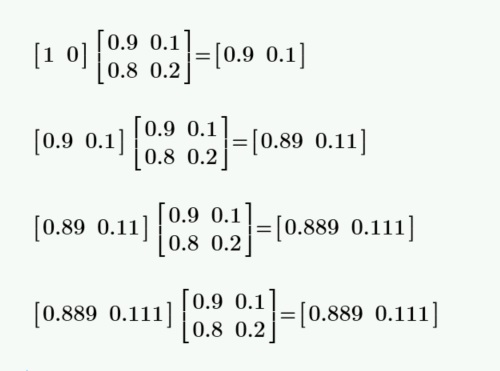
There are three mathematical ways to calculate the Steady-State Probability. Below shown the P matrix can be multiplied by itself to get the transition probabilities matrix.


The second way is the way to take account of the starting state that contributes to time-dependent probabilities.
State Probability Time Interval
| Time Interval | State Operation | State Failed |
| 0 | 0.9 | 0.2 |
| 1 | 0.89 | 0.12 |
| 2 | 0.889 | 0.112 |
| 3 | 0.889 | 0.111 |
| 4 | 0.889 | 0.111 |
The last stage is known as the limiting state probability or Steady-Stage Probability which the top and bottom rows of the limiting state probability matrix are the same numbers. And the Steady State of Availability is 0.889.
The third method used the direct algebraic method which offers the quickest solution to Limiting State Probability or Steady State Probability State. This technique is called the “regular” Markov model.

